Note: This post is an English adaptation of my original Chinese article (URL). Some parts have been modified for clarity, cultural relevance, or to better fit the English-speaking audience.
I have also pondered this question and will now present an answer from a higher-level perspective, serving as a personal note. I welcome any corrections for potential errors or issues. Thank you!
First, we must clarify one point:
The term “Phasor” is derived from “Phase Vector.” From a mathematical standpoint, a phasor is essentially a complex number. A complex number is also a vector (a fact that can be verified by proving that the set of complex numbers $\mathbb{C}$, along with the operations of complex addition and scalar multiplication, constitutes a vector space over the field of real numbers $\mathbb{R}$). Therefore, a phasor is also a vector. However, when we discuss phasors, we are typically emphasizing their representation in the form of a complex number.
So, can phasors be introduced when analyzing any AC circuit?
This requires a case-by-case analysis. Most importantly:
- If the AC circuit contains non-linear electrical components (defined as components for which the operator relating their $I(t)$ and $V(t)$ lacks the property of linearity), such as a diode, then we cannot use phasors at all. Therefore, phasor analysis is only applicable to linear AC circuits.
- If the AC circuit contains time-variant electrical components (defined as components for which the operator relating their $I(t)$ and $V(t)$ lacks the property of time-invariance), such as a time-varying resistor, we also cannot use phasors. Therefore, phasor analysis is only applicable to time-invariant AC circuits.
(Incidentally, an operator is also a function, but the term ‘operator’ typically refers to a function that maps one function space to another.)
Combining these two points, we can conclude that an AC circuit must at least satisfy the properties of being Linear Time-Invariant (commonly abbreviated as LTI; hereafter, I will use “LTI AC circuit” to denote an AC circuit that is LTI) for phasors to be applicable. The reason for this will be explained below.
Furthermore, we must agree upon two additional points: first, that for any circuit, the operator relating $I(t)$ and $V(t)$ for each electrical component is a real operator (an equivalent statement is that the operator commutes with complex conjugation), and second, that an AC circuit must have external sources, and all such sources must be real-valued. These additional definitions for circuits and AC circuits are necessary because the conditions $\Lambda_1$ and $\Lambda_3$ will be utilized in the mathematical proof that follows.
So, why introduce phasors when analyzing LTI AC circuits?
Because it simplifies the analysis.
And why does using phasors simplify the analysis of LTI AC circuits?
When analyzing LTI AC circuits, such as RLC circuits, what we are actually doing is “solving the system of KCL and KVL equations for the circuit.” This is entirely equivalent to “solving the state-space equations of the LTI system.“
Mathematically, this equivalence is expressed as:
$$
\begin{cases} \mathbf{T_I} \mathbf{I}(t) = \mathbf{S_I}(t) &\text{(KCL)} \\ \mathbf{T_V} \mathbf{V}(t) = \mathbf{S_V}(t) &\text{(KVL)} \end{cases} \quad \Longleftrightarrow \quad \begin{cases} \mathbf{\dot{x}}(t) = \mathbf{A}\mathbf{x}(t) + \mathbf{B}\mathbf{u}(t) & \text{(State)} \\ \mathbf{y}(t) = \mathbf{C}\mathbf{x}(t) + \mathbf{D}\mathbf{u}(t) & \text{(Output)} \end{cases}
$$
Where:
- $I(t)$ is the real-valued vector of currents through each electrical component in the circuit.
- $V(t)$ is the real-valued vector of voltages across each electrical component in the circuit.
- $T_I$ and $T_V$ are Ternary Matrices (or Signed Incidence Matrices), whose elements can take values from $\{-1, 0, 1\}$.
- $S_I(t)$ and $S_V(t)$ are real-valued vectors whose elements can be $\{\pm I_y(t), 0\}$ and $\{\pm V_z(t), 0\}$ respectively, where $I_y(t)$ and $V_z(t)$ represent the currents and voltages supplied by the external sources $y,z$ in the circuit.
- $x(t)$ is the state variable vector.
- $u(t)$ is the input vector, which contains the currents and voltages from all external sources $y,z$.
- $y(t)$ is the output vector.
- $A, B, C, D$ are real-valued matrices.
With this foundation, let us return to our question: why do phasors simplify the analysis of LTI AC circuits?
Because a phasor is a complex number, we can use Euler’s formula ($e^{j\theta}=\cos(\theta)+j\sin(\theta)$) to convert between its polar and Cartesian forms. As mentioned, our goal is to solve the State-Space Equations. Based on the following conditions:
- $\Lambda_1$: $A, B, C, D$ are real-valued matrices.
- $\Lambda_2$: Euler’s formula.
- $\Lambda_3$: The currents and voltages of all electrical components in the AC circuit are sinusoidal functions of the same frequency. (Even if the external sources in the AC circuit have different frequencies, the Superposition Principle can be applied to analyze each frequency component separately, with the final result obtained by summing the individual results. Therefore, this assumption does not result in a loss of generality.)
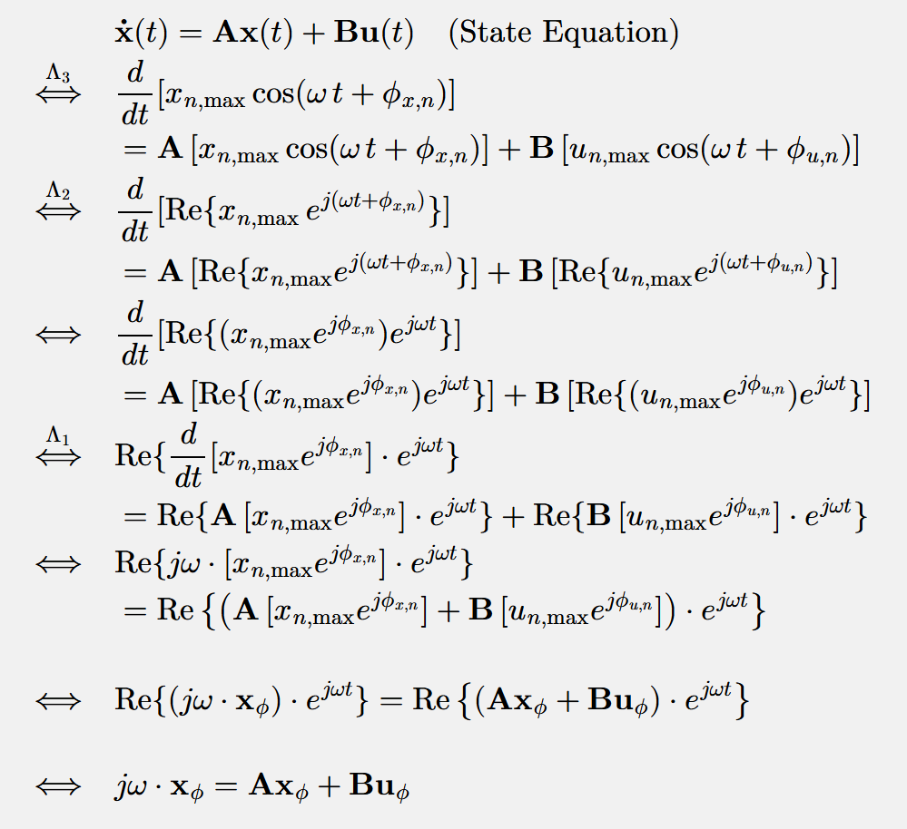
Given that the source inputs are of the form $I_{y}(t)= I_{y, \max}\cos(\omega\, t + \phi_{y})$ and $V_{z}(t)= V_{z, \max}\cos(\omega\, t + \phi_{z})$, we can then assume that the elements within the state vector $x$ have the form $x_n(t) =x_{n, \max}\cos(\omega\, t + \phi_{x,n})$ and the elements within the input vector $u$ have the form $u_n(t) =u_{n, \max}\cos(\omega\, t + \phi_{u,n})$. This allows for the following proof (in the derivation below, $[a_n]$ denotes a vector whose elements are $a_n$, where $n$ is the row index):
\begin{aligned}
& \mathbf{\dot{x}}(t) = \mathbf{A}\mathbf{x}(t) + \mathbf{B}\mathbf{u}(t) \quad \text{(State Equation)} \\
\overset{\Lambda _3}{\Longleftrightarrow} \quad & \dfrac{d}{dt}[x_{n, \max}\cos(\omega\, t + \phi_{x,n})] \\
& = \mathbf{A} \, [x_{n, \max}\cos(\omega\, t + \phi_{x,n})] + \mathbf{B} \, [u_{n, \max}\cos(\omega\, t + \phi_{u,n})] \\
\overset{\Lambda _2}{\Longleftrightarrow} \quad & \dfrac{d}{dt}[\text{Re}\{x_{n,\max} \, e^{j (\omega t+\phi_{x,n})}\}] \\
& = \mathbf{A} \, [\text{Re}\{x_{n, \max}e^{j (\omega t+\phi_{x,n})}\}] + \mathbf{B} \, [ \text{Re} \{u_{n, \max}e^{j (\omega t+\phi_{u,n})}\}] \\
\Longleftrightarrow \quad & \dfrac{d}{dt}[\text{Re}\{ (x_{n,\max} e^{j\phi_{x,n}}) e^{j\omega t}\}] \\
& = \mathbf{A} \, [ \text{Re}\{ (x_{n,\max} e^{j\phi_{x,n}}) e^{j\omega t} \}] + \mathbf{B} \, [ \text{Re} \{ (u_{n,\max} e^{j\phi_{u,n}}) e^{j\omega t} \}] \\
\overset{\Lambda _1}{\Longleftrightarrow} \quad & \text{Re}\{ \dfrac{d}{dt}[x_{n,\max} e^{j\phi_{x,n}} ] \cdot e^{j\omega t} \} \\
& = \text{Re}\{ \mathbf{A} \, [ x_{n,\max} e^{j\phi_{x,n}} ] \cdot e^{j\omega t} \} + \text{Re} \{ \mathbf{B} \, [ u_{n,\max} e^{j\phi_{u,n}} ] \cdot e^{j\omega t} \} \\
\Longleftrightarrow \quad & \text{Re} \{ j\omega \cdot [x_{n,\max} e^{j\phi_{x,n}} ] \cdot e^{j\omega t} \} \\
& = \text{Re} \left \{ \left ( \mathbf{A} \, [ x_{n,\max} e^{j\phi_{x,n}} ] + \mathbf{B} \, [ u_{n,\max} e^{j\phi_{u,n}}] \right ) \cdot e^{j\omega t} \right \} \\
\\
\Longleftrightarrow \quad & \text{Re} \{ \left ( j\omega \cdot \mathbf{x}_{\phi} \right ) \cdot e^{j\omega t} \} = \text{Re} \left \{ \left ( \mathbf{A} \mathbf{x}_{\phi} + \mathbf{B} \mathbf{u}_{\phi} \right ) \cdot e^{j\omega t} \right \} \\
\\
\Longleftrightarrow \quad & j\omega \cdot \mathbf{x}_{\phi} = \mathbf{A} \mathbf{x}_{\phi} + \mathbf{B} \mathbf{u}_{\phi}
\end{aligned}
Here, $\mathbf{x}_{\phi}$ and $\mathbf{u}_{\phi}$ are the phasor representations of the state and input vectors, respectively (e.g., $\mathbf{x}_{\phi} = [x_{n,\max}e^{j\phi_{x,n}}]$).
As can be seen, by introducing phasors, we have transformed the State Equation, a system of differential equations, into a system of algebraic equations. The Output Equation is already an algebraic system and thus requires no transformation.
In other words, we have equivalently transformed the problem from “solving a system of differential equations $+$ algebraic equations” to “solving a system of purely algebraic equations,” which significantly reduces the difficulty.
Regarding the imaginary part of a phasor, does it have physical significance?
On this point, I am actually uncertain, as I do not know the rigorous physical definition of what it means for a number to “have physical significance.”
Leave a Reply