Author: Louis Liu

Can Lorentz Transformations Be Derived from General Relativity?

Note: This post is an English adaptation of my original Chinese article (URL). Some parts have been modified for clarity, cultural relevance, or to better fit the English-speaking audience.

Update:

After reading another article, I realized that I had initially misinterpreted the question. I had understood the term “derive” in its strict mathematical sense, implying a proof without any additional assumptions. Consequently, when I attempted to derive the properties of Special Relativity (SR) directly from the definitional properties (or axioms) of General Relativity (GR) without setting assumptions such as a flat manifold, I concluded that GR cannot derive SR. From a physics perspective, this conclusion is somewhat flawed, and upon reflection, I found it unsatisfactory. I apologize for the initial oversight and will now correct my original answer.

In retrospect, framing the question as “Can GR be reduced to SR?” is more appropriate than “Can GR derive SR?” The term “reduce” better emphasizes the process of derivation under a specific set of conditions and constraints.

The specific conditions required for GR to reduce to SR are the assumptions of a “Lorentzian manifold” and “flatness (as the Riemann curvature tensor is zero everywhere, also known as local flatness)“. With these two conditions, it can be shown that a neighborhood of any point on the manifold is isometric to Minkowski space. This is how a local version of SR is derived.

Original Answer:

The framework of Special Relativity (SR) incorporates the Minkowski metric as a fundamental axiom to guarantee the “constancy of the speed of light in all inertial reference frames.”

The framework of General Relativity (GR), however, does not stipulate the Minkowski metric as an axiom. GR only requires that its metric satisfy the axioms internal to GR; therefore, the metric in GR is not necessarily the Minkowski metric. Therefore, GR cannot be used to derive SR.
Why Do Some Forces like Friction Not Satisfy Time-Reversal Symmetry?

Note: This post is an English adaptation of my original Chinese article (URL). Some parts have been modified for clarity, cultural relevance, or to better fit the English-speaking audience.

This question is functionally equivalent to Loschmidt’s Paradox, also known as the reversibility paradox. At its core, it addresses a fundamental conflict in physics.

The fundamental mechanical equations for a single particle in classical mechanics are symmetric under time reversal. Consequently, the evolution of an entire system of particles should also be time-reversal symmetric and, therefore, perfectly reversible. However, according to Boltzmann’s H-theorem (which is a specific instance of the second law of thermodynamics, though not as general) the entropy of a particle system is overwhelmingly likely to not decrease. While entropy reduction is possible, its probability is infinitesimally small. This implies that the evolution of the particle system is not time-reversal symmetric, so it is irreversible. This presents a direct contradiction.

Later, in his response to Loschmidt’s critique, Boltzmann acknowledged that his proof of the H-theorem introduced the “molecular chaos” assumption (which is called “Stosszahlansatz”). More precisely, this assumption was intrinsically embedded in the construction of the Boltzmann equation, from which the H-theorem is derived. This assumption, by its mathematical nature, lacks time-reversal symmetry, and as a result, the Boltzmann equation itself does not possess this property.

Does this imply that, without the molecular chaos assumption, one could construct an equation that does satisfy time-reversal symmetry to describe the state of a particle system? Indeed, this is the case. The Liouville equation is a perfect example of such an equation, and it is fully time-reversal symmetric.

However, the crucial issue is that “reversibility” in the context of the paradox has distinct meanings: microscopic reversibility and thermodynamic reversibility. These two concepts are fundamentally different. Time-reversal symmetry is equivalent to microscopic reversibility, but it does not imply thermodynamic (or macroscopic) reversibility. Time-reversal symmetry and microscopic reversibility concern the possibility of reverse evolution, whereas thermodynamic reversibility concerns the probability of a macroscopic state evolving in reverse.

Microscopic reversibility physically means that “the probability of a system’s forward evolution is non-zero if and only if the probability of its reverse evolution is non-zero.” Mathematically, this is expressed as $P_F[ A \to B] \ne 0 \Longleftrightarrow P_R[B \to A] \ne 0$. In contrast, thermodynamic reversibility physically means that “the probability of the system’s forward evolution is equal to the probability of its reverse evolution,” expressed mathematically as $P_F[A \to B] = P_R[B \to A]$. These definitions are derived from the Crooks fluctuation theorem. For those interested, this theorem can be used to derive the Jarzynski equality, which, when combined with Jensen’s inequality, yields the Clausius statement of the second law of thermodynamics. Therefore, a process can be defined as irreversible as long as “the probability of the forward evolution is greater than the probability of the reverse evolution,” although typically we require that the forward probability be substantially greater.
Why is the Lorentz Transformation Linear, and How is its Linearity Derived?

Note: This post is an English adaptation of my original Chinese article (URL). Some parts have been modified for clarity, cultural relevance, or to better fit the English-speaking audience.

If physical and historical factors are disregarded and the question is considered from a purely mathematical standpoint, the linearity of the Lorentz transformation can be established as follows:

Assume the physical universe is a flat, complete, and simply connected pseudo-Riemannian manifold. Such a manifold must be isometric to a pseudo-Euclidean space. Consequently, any isometry of this manifold must be an affine transformation.

If this pseudo-Riemannian manifold is endowed with the Minkowski metric, its isometries are precisely the Poincaré transformations. The linear part of any Poincaré transformation is a Lorentz transformation.

The selection of the Minkowski metric is predicated on its mathematical convenience. From a historical perspective, however, the formalization of Minkowski space occurred after Lorentz had proposed his transformations and Einstein had published the theory of Special Relativity. The impetus for Minkowski’s formulation of spacetime was his discovery that the quantity known as the spacetime interval remains invariant under the Lorentz transformation. Subsequently, to systematically handle transformations between arbitrary inertial reference frames within Special Relativity, Minkowski defined Minkowski spacetime based on this principle of “spacetime interval invariance.”

The requirement for isometries, subsequent to adopting the Minkowski metric, stems from the fact that transformations preserving this metric inherently satisfy the two fundamental postulates of Special Relativity: “The laws of physics are the same in all inertial frames of reference” and “The speed of light in a vacuum has the same value in all inertial frames of reference.”

As to why the Lorentz transformation (a linear transformation) is more widely recognized and emphasized in the context of Special Relativity than the Poincaré transformation (an affine transformation), it is most likely because the Lorentz component directly leads to the derivation of canonical relativistic phenomena such as time dilation and length contraction. In contrast, the translational component of the Poincaré transformation can appear trivial. Nevertheless, the Poincaré transformation represents the most general isometry within Minkowski spacetime.
Given the scientific consensus on the principle of the constancy of the speed of light, is it possible that the speed of light is, in fact, variable, and this has simply not yet been observed?

Note: This post is an English adaptation of my original Chinese article (URL). Some parts have been modified for clarity, cultural relevance, or to better fit the English-speaking audience.

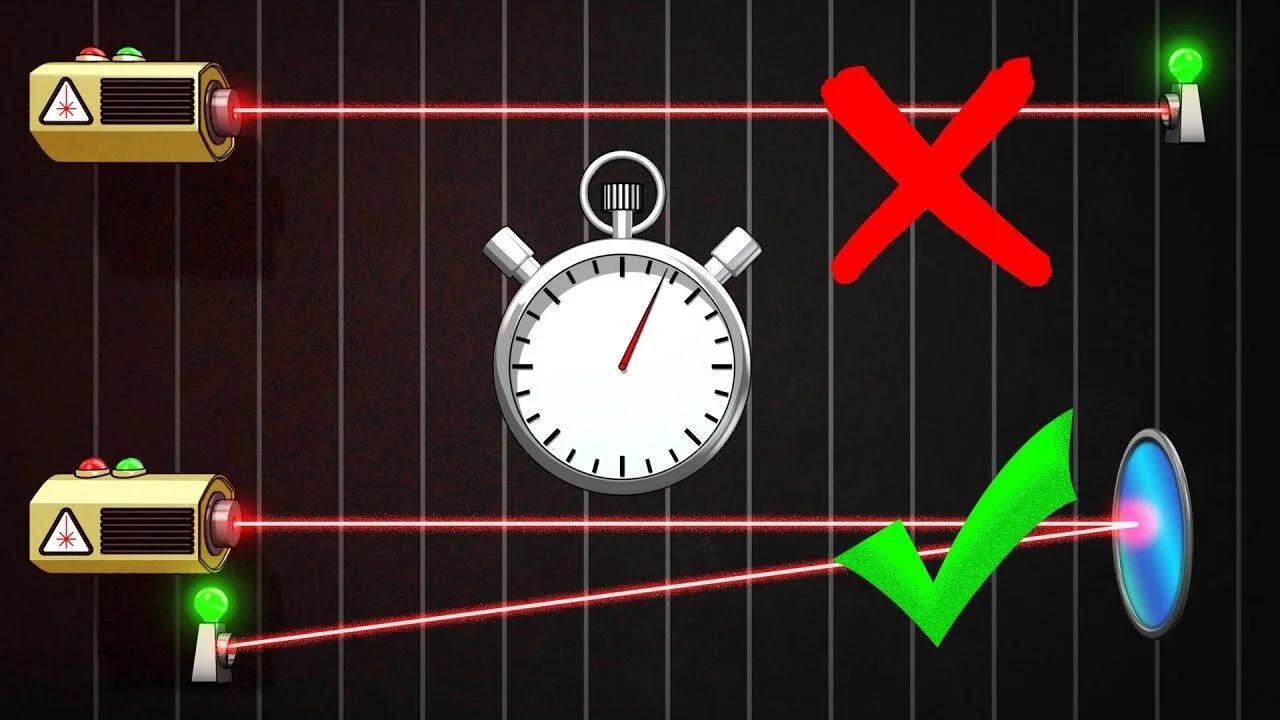
The Veritasium channel discussed the question of whether the speed of light is constant in one of its videos (here), where it highlighted the following fact: In essence, all direct measurements of the speed of light are measurements of its round-trip speed, because the one-way speed of light is not directly measurable.

The mathematical proof for this conclusion was provided by Hans Reichenbach. In essence, by positing that the moment light completes a one-way path is $t_2=t_1+\varepsilon (t_3-t_1)$, where $0 < \varepsilon < 1$, $t_1$ is the start time, $t_3$ is the time when the light completes its return journey, and $c$ is the constant for the round-trip speed of light, he demonstrated that:

$$ \left\{\begin{matrix} c_{\to} = & \dfrac{c}{2 \varepsilon } \\ c_{\gets} = & \dfrac{c}{2 (1-\varepsilon ) } \end{matrix}\right. $$

From this, it is evident that, fundamentally, no physical experiment can measure the one-way speed of light. However, for the sake of simplicity, Albert Einstein, in his theory of relativity, adopted $\varepsilon = \dfrac{1}{2}$ to obtain $c_{\to} = c_{\gets} = c$. This formulation possesses significant symmetry and simplicity, making its acceptance by the physics community a logical consequence.

A user in the comments section (of my original Chinese article) proposed a profound idea: “This is based on synchronizing clocks using light signals. If two clocks, synchronized at the same point, are then slowly moved to two different locations, could this method be used for measurement?“

This is an excellent thought! However, it is unfortunately still not feasible. This is because after two clocks are synchronized, if one is moved away at a slow, constant velocity ($v$) to a distance ($L$), the effects of time dilation must be considered. However, the Lorentz factor in the time dilation formula used in modern physics itself incorporates the one-way speed of light, $\textcolor{red}{c}$. This implies that the measurement formula in your proposed experiment is inherently dependent on the value of the one-way speed of light $\Big($the time difference between the two clocks in the calculation is $\Delta t_{delay} = \Delta t\,(1-\textcolor{red}{\gamma}) = \dfrac{L}{v}\,\left (1-\sqrt{1-\dfrac{v^2}{\textcolor{red}{c}^2}} \right )$$\Big)$, which leads to the problem of circular reasoning. If you were to adopt Reichenbach’s convention and derive your own formula for time dilation for use in your hypothetical experiment, it would still contain the value $\varepsilon$, which you must presuppose. Therefore, the circular argument cannot be circumvented.
Why are Differential Equations in Physics Typically at Most Second-Order?

Note: This post is an English adaptation of my original Chinese article (URL). Some parts have been modified for clarity, cultural relevance, or to better fit the English-speaking audience.

This is a compelling question, and the explanation is rooted in a fundamental principle of physical systems and a key mathematical theorem. The essential reason is as follows:

The energy of any non-degenerate physical system must possess a lower bound. Let us designate this as postulate $\Psi$. This principle is regarded as an empirical conclusion derived from consistent experimental observation.

There exists a mathematical theorem known as Ostrogradsky’s Instability. It states that if the Lagrangian ($L$) of any non-degenerate system depends on time derivatives of the generalized coordinates of an order higher than one (e.g., $\ddot{q}$), then the Hamiltonian of the system is necessarily unbounded from below.

By applying the contrapositive of Ostrogradsky’s theorem in conjunction with postulate $\Psi$, we can deduce a critical constraint: The Lagrangian of any stable, non-degenerate physical system must not depend on second or higher-order time derivatives of its generalized coordinates. The Lagrangian must be a function of the form $L(q, \dot{q}, t)$.

Furthermore, the conventional definitions of potential energy and kinetic energy in physics also conform to the constraint that their derivative to generalized coordinate and generalized velocity is 0th-order respectively.

Therefore, the Euler-Lagrange equations of motion for any such non-degenerate physical system will be second-order (at most) differential equations.
Why are Phasors Introduced in Circuit Analysis, and What is the Physical Significance of Their Components?
Note: This post is an English adaptation of my original Chinese article (URL). Some parts have been modified for clarity, cultural relevance, or to better fit the English-speaking audience.

I have also pondered this question and will now present an answer from a higher-level perspective, serving as a personal note. I welcome any corrections for potential errors or issues. Thank you!

First, we must clarify one point:
The term “Phasor” is derived from “Phase Vector.” From a mathematical standpoint, a phasor is essentially a complex number. A complex number is also a vector (a fact that can be verified by proving that the set of complex numbers $\mathbb{C}$, along with the operations of complex addition and scalar multiplication, constitutes a vector space over the field of real numbers $\mathbb{R}$). Therefore, a phasor is also a vector. However, when we discuss phasors, we are typically emphasizing their representation in the form of a complex number.

So, can phasors be introduced when analyzing any AC circuit?

This requires a case-by-case analysis. Most importantly:
- If the AC circuit contains non-linear electrical components (defined as components for which the operator relating their $I(t)$ and $V(t)$ lacks the property of linearity), such as a diode, then we cannot use phasors at all. Therefore, phasor analysis is only applicable to linear AC circuits.
- If the AC circuit contains time-variant electrical components (defined as components for which the operator relating their $I(t)$ and $V(t)$ lacks the property of time-invariance), such as a time-varying resistor, we also cannot use phasors. Therefore, phasor analysis is only applicable to time-invariant AC circuits.
(Incidentally, an operator is also a function, but the term ‘operator’ typically refers to a function that maps one function space to another.)

Combining these two points, we can conclude that an AC circuit must at least satisfy the properties of being Linear Time-Invariant (commonly abbreviated as LTI; hereafter, I will use “LTI AC circuit” to denote an AC circuit that is LTI) for phasors to be applicable. The reason for this will be explained below.

Furthermore, we must agree upon two additional points: first, that for any circuit, the operator relating $I(t)$ and $V(t)$ for each electrical component is a real operator (an equivalent statement is that the operator commutes with complex conjugation), and second, that an AC circuit must have external sources, and all such sources must be real-valued. These additional definitions for circuits and AC circuits are necessary because the conditions $\Lambda_1$ and $\Lambda_3$ will be utilized in the mathematical proof that follows.

So, why introduce phasors when analyzing LTI AC circuits?

Because it simplifies the analysis.

And why does using phasors simplify the analysis of LTI AC circuits?

When analyzing LTI AC circuits, such as RLC circuits, what we are actually doing is “solving the system of KCL and KVL equations for the circuit.” This is entirely equivalent to “solving the state-space equations of the LTI system.“
Mathematically, this equivalence is expressed as:

$$
\begin{cases} \mathbf{T_I} \mathbf{I}(t) = \mathbf{S_I}(t) &\text{(KCL)} \\ \mathbf{T_V} \mathbf{V}(t) = \mathbf{S_V}(t) &\text{(KVL)} \end{cases} \quad \Longleftrightarrow \quad \begin{cases} \mathbf{\dot{x}}(t) = \mathbf{A}\mathbf{x}(t) + \mathbf{B}\mathbf{u}(t) & \text{(State)} \\ \mathbf{y}(t) = \mathbf{C}\mathbf{x}(t) + \mathbf{D}\mathbf{u}(t) & \text{(Output)} \end{cases}
$$

Where:
- $I(t)$ is the real-valued vector of currents through each electrical component in the circuit.
- $V(t)$ is the real-valued vector of voltages across each electrical component in the circuit.
- $T_I$ and $T_V$ are Ternary Matrices (or Signed Incidence Matrices), whose elements can take values from $\{-1, 0, 1\}$.
- $S_I(t)$ and $S_V(t)$ are real-valued vectors whose elements can be $\{\pm I_y(t), 0\}$ and $\{\pm V_z(t), 0\}$ respectively, where $I_y(t)$ and $V_z(t)$ represent the currents and voltages supplied by the external sources $y,z$ in the circuit.
- $x(t)$ is the state variable vector.
- $u(t)$ is the input vector, which contains the currents and voltages from all external sources $y,z$.
- $y(t)$ is the output vector.
- $A, B, C, D$ are real-valued matrices.
With this foundation, let us return to our question: why do phasors simplify the analysis of LTI AC circuits?

Because a phasor is a complex number, we can use Euler’s formula ($e^{j\theta}=\cos(\theta)+j\sin(\theta)$) to convert between its polar and Cartesian forms. As mentioned, our goal is to solve the State-Space Equations. Based on the following conditions:
- $\Lambda_1$: $A, B, C, D$ are real-valued matrices.
- $\Lambda_2$: Euler’s formula.
- $\Lambda_3$: The currents and voltages of all electrical components in the AC circuit are sinusoidal functions of the same frequency. (Even if the external sources in the AC circuit have different frequencies, the Superposition Principle can be applied to analyze each frequency component separately, with the final result obtained by summing the individual results. Therefore, this assumption does not result in a loss of generality.)
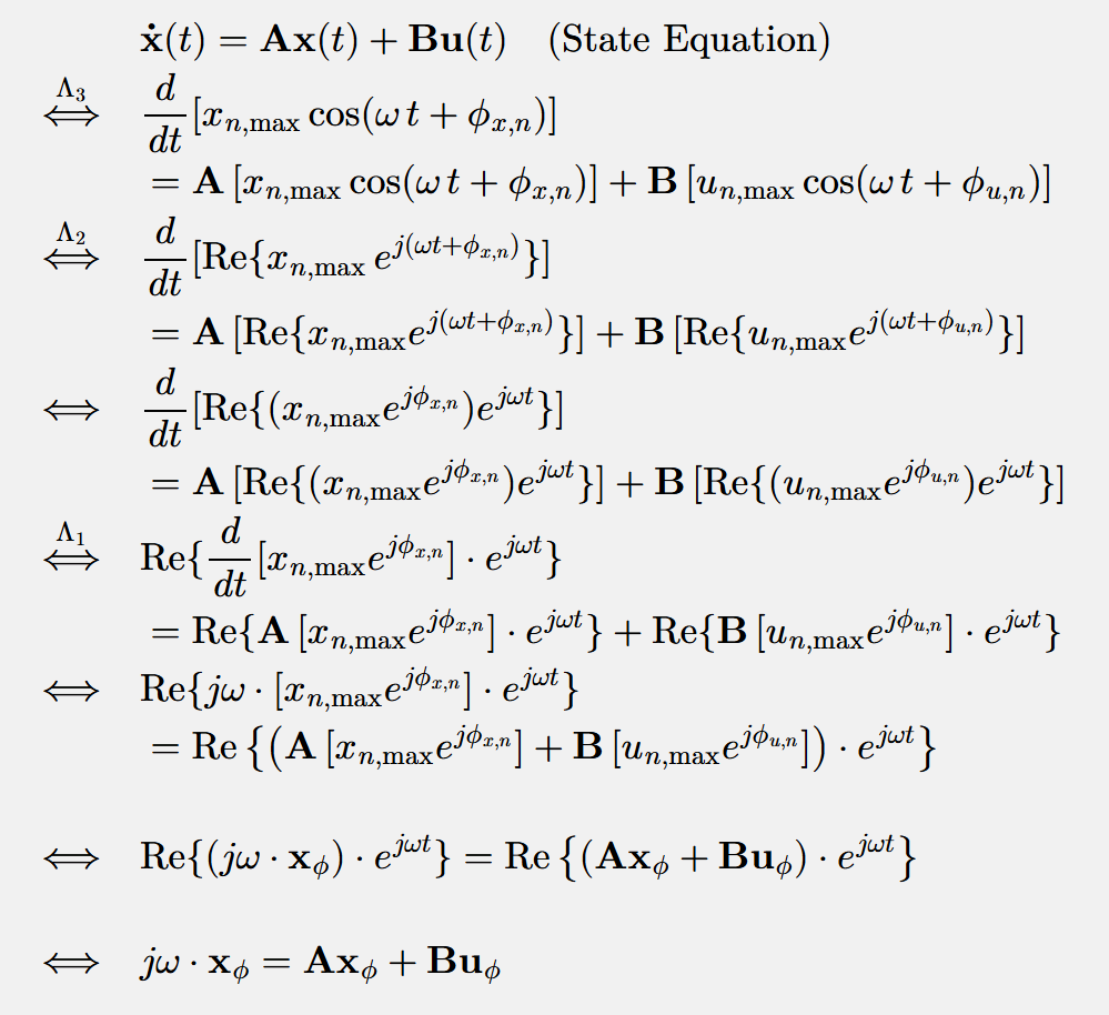
Given that the source inputs are of the form $I_{y}(t)= I_{y, \max}\cos(\omega\, t + \phi_{y})$ and $V_{z}(t)= V_{z, \max}\cos(\omega\, t + \phi_{z})$, we can then assume that the elements within the state vector $x$ have the form $x_n(t) =x_{n, \max}\cos(\omega\, t + \phi_{x,n})$ and the elements within the input vector $u$ have the form $u_n(t) =u_{n, \max}\cos(\omega\, t + \phi_{u,n})$. This allows for the following proof (in the derivation below, $[a_n]$ denotes a vector whose elements are $a_n$, where $n$ is the row index):

\begin{aligned}
& \mathbf{\dot{x}}(t) = \mathbf{A}\mathbf{x}(t) + \mathbf{B}\mathbf{u}(t) \quad \text{(State Equation)} \\
\overset{\Lambda _3}{\Longleftrightarrow} \quad & \dfrac{d}{dt}[x_{n, \max}\cos(\omega\, t + \phi_{x,n})] \\
& = \mathbf{A} \, [x_{n, \max}\cos(\omega\, t + \phi_{x,n})] + \mathbf{B} \, [u_{n, \max}\cos(\omega\, t + \phi_{u,n})] \\
\overset{\Lambda _2}{\Longleftrightarrow} \quad & \dfrac{d}{dt}[\text{Re}\{x_{n,\max} \, e^{j (\omega t+\phi_{x,n})}\}] \\
& = \mathbf{A} \, [\text{Re}\{x_{n, \max}e^{j (\omega t+\phi_{x,n})}\}] + \mathbf{B} \, [ \text{Re} \{u_{n, \max}e^{j (\omega t+\phi_{u,n})}\}] \\
\Longleftrightarrow \quad & \dfrac{d}{dt}[\text{Re}\{ (x_{n,\max} e^{j\phi_{x,n}}) e^{j\omega t}\}] \\
& = \mathbf{A} \, [ \text{Re}\{ (x_{n,\max} e^{j\phi_{x,n}}) e^{j\omega t} \}] + \mathbf{B} \, [ \text{Re} \{ (u_{n,\max} e^{j\phi_{u,n}}) e^{j\omega t} \}] \\
\overset{\Lambda _1}{\Longleftrightarrow} \quad & \text{Re}\{ \dfrac{d}{dt}[x_{n,\max} e^{j\phi_{x,n}} ] \cdot e^{j\omega t} \} \\
& = \text{Re}\{ \mathbf{A} \, [ x_{n,\max} e^{j\phi_{x,n}} ] \cdot e^{j\omega t} \} + \text{Re} \{ \mathbf{B} \, [ u_{n,\max} e^{j\phi_{u,n}} ] \cdot e^{j\omega t} \} \\
\Longleftrightarrow \quad & \text{Re} \{ j\omega \cdot [x_{n,\max} e^{j\phi_{x,n}} ] \cdot e^{j\omega t} \} \\
& = \text{Re} \left \{ \left ( \mathbf{A} \, [ x_{n,\max} e^{j\phi_{x,n}} ] + \mathbf{B} \, [ u_{n,\max} e^{j\phi_{u,n}}] \right ) \cdot e^{j\omega t} \right \} \\
\\
\Longleftrightarrow \quad & \text{Re} \{ \left ( j\omega \cdot \mathbf{x}_{\phi} \right ) \cdot e^{j\omega t} \} = \text{Re} \left \{ \left ( \mathbf{A} \mathbf{x}_{\phi} + \mathbf{B} \mathbf{u}_{\phi} \right ) \cdot e^{j\omega t} \right \} \\
\\
\Longleftrightarrow \quad & j\omega \cdot \mathbf{x}_{\phi} = \mathbf{A} \mathbf{x}_{\phi} + \mathbf{B} \mathbf{u}_{\phi}
\end{aligned}

Here, $\mathbf{x}_{\phi}$ and $\mathbf{u}_{\phi}$ are the phasor representations of the state and input vectors, respectively (e.g., $\mathbf{x}_{\phi} = [x_{n,\max}e^{j\phi_{x,n}}]$).

As can be seen, by introducing phasors, we have transformed the State Equation, a system of differential equations, into a system of algebraic equations. The Output Equation is already an algebraic system and thus requires no transformation.

In other words, we have equivalently transformed the problem from “solving a system of differential equations $+$ algebraic equations” to “solving a system of purely algebraic equations,” which significantly reduces the difficulty.

Regarding the imaginary part of a phasor, does it have physical significance?

On this point, I am actually uncertain, as I do not know the rigorous physical definition of what it means for a number to “have physical significance.”

My Fall 2025 U.S. Transfer Admissions Decisions (Undergraduate)

Note: This post is an English adaptation of my original Chinese article (URL). Some parts have been modified for clarity, cultural relevance, or to better fit the English-speaking audience.

As of May 18, 2025, all the transfer decisions from the universities I applied to have been released. Fortunately, at the very last moment, the outcome was positive, although the journey was quite tumultuous.

First, allow me to provide my basic information:
Male, not LGBTQ+, international student, non-citizen without a green card, not a first-generation student. My MBTI is INTJ. I handled the entire transfer application process myself (DIY). I am currently enrolled at a Top 100 university, majoring in Pure Mathematics (all my transfer applications were for Pure Math as well). I have no SAT score, no competition awards, a university GPA of 3.99, and a high school GPA equivalent to somewhere in the 2.x range. I will not disclose further information to avoid being identified by acquaintances.

Decision Date	University	Outcome
4/4	UC Irvine	❌
4/18	UC Berkeley	⏰
4/23	UC Santa Barbara	✅
4/25	UC San Diego	✅
4/25	UC Los Angeles	✅
4/26	Caltech	❌
5/6	Princeton	❌
5/9	Stanford	❌
5/15	Cornell	❌
5/18	Carnegie Mellon University	✅

Before the CMU decision was released, it was truly disheartening to see the rejections come in one by one from UC Berkeley and the private universities. However, it also felt justifiable. After all, I had no SAT score, no competition awards, and a poor high school GPA. If they had admitted me, what would that have said to the students who had genuinely worked hard for years in high school?

Occasionally, I would imagine: if I hadn’t been addicted to video games in high school, if I hadn’t gone through that period of confusion, and had just continued to study for the sake of studying without understanding why, would my results be better today? My family and I both believe that under those circumstances, I might have found myself in an even more dire situation upon entering university, perhaps even facing academic suspension.

You see, my academic performance was actually decent when I was younger. However, this was primarily due to various external motivating factors, such as not wanting to disappoint my family and teachers, coupled with a genuine interest in some subjects. Nevertheless, I still didn’t understand the fundamental purpose of learning; I viewed it merely as a task that every peer was striving to complete. Consequently, as soon as I finished my homework, I would play video games. My parents weren’t overly strict; as long as my grades were acceptable, they allowed me this freedom.

However, things changed when I entered the international division of my high school. I had my own phone and computer, and the curriculum emphasized self-discipline, with no homeroom teacher constantly monitoring me. Without these restraints, I completely let myself go. At that time, I paid no attention to my GPA. My homework was often done carelessly, just to get by. During class, I frequently played games in the back row (and to be honest, I was quite unskilled at them, but my lack of skill didn’t diminish my desire to play). Even my previous passion for certain subjects could not compete with the allure of gaming. As a result, when it came time to apply for undergraduate studies in the US, my GPA was absurdly low. I was lost, with no idea what I wanted to do in the future or what the purpose of my life was. To make matters worse, I was so unconcerned about my future that I even missed the application deadlines for all the University of California campuses. Fortunately, a kind university eventually took me in.

Later, determined not to become a dependent living off my parents, I proceeded to study abroad. After some time, I discovered that I was indeed capable of performing well academically, and my GPA returned to a normal, high level. Subsequently, through experiencing loneliness and dedicating myself to serious research in certain areas, I matured. I began to realize what I wanted, the kind of person I wanted to become, and most importantly, I came to understand why I study and how to study effectively.

The rest of the story is one of getting back on track. For instance, I engaged in some undergraduate research, completed numerous projects and activities, and cultivated strong relationships with my professors. Following this, applying for a transfer was the logical next step.

Returning to the main point, my top choice for transfer from the very beginning was actually CMU. Some might argue that CMU’s pure mathematics program cannot compare to those at Princeton, Stanford, etc., and may even seem inferior to UCLA’s. However, the field of Pure Mathematics is divided into many sub-disciplines, and in my specific area of interest, CMU’s program is considered Tier 1. Therefore, the conclusion to this story is, for me, quite perfect.

And so, my story ends here. I hope that all of you can also get into your dream schools. Even if you don’t, please do not be discouraged, because your future is not defined by this single setback. Keep going!

Intro to Generalized Coordinates
Note: This post is an English adaptation of my original Chinese article (URL). Some parts have been modified for clarity, cultural relevance, or to better fit the English-speaking audience.

When you first started learning analytical mechanics, have you ever been confused about what generalized coordinates really are? Are they just “generalized” versions of Cartesian coordinates? How general can they be?

In essence, generalized coordinates are a set of parameterized, irreducible, and independent variables that can fully describe every possible state of a mechanical system subject to various constraints. (Here, “irreducible” basically means “minimal,” implying that the number of these coordinates is exactly what is needed to completely describe the system under its constraints. If you have more coordinates than that, the set contains dependent coordinates; if you have fewer, you cannot fully describe the system.)

So, what’s the difference compared to Cartesian coordinates? It may seem that generalized coordinates only add “parameterization” and “irreducibility” as properties.

But let’s clarify one point first: both generalized coordinates and Cartesian coordinates can “fully describe the system’s motion under constraints.” Why then do we even need generalized coordinates in analytical mechanics? Is it because Cartesian coordinates are not sufficient? Or are those extra properties — “parameterization” and “irreducibility” — really that crucial? Let’s take an example to answer these questions.

Assume we have a classical mechanical system with $N$ particles in $D$ dimensions, subject to $M$ constraint equations. (We assume the system is “well-behaved,” meaning all constraints are integrable, independent, etc. We’ll use Newtonian mechanics for our discussion to highlight the difference between generalized and Cartesian coordinates.)
- Using Cartesian coordinates: we first write down all the force-component equations for each particle, then add these $M$ constraint equations, leading to a total of $N \times D + M$ equations to solve.
- Using generalized coordinates: we would first apply some parameterization methods, incorporating the known constraint equations to determine a set of generalized coordinates. After that, we only need to write down the force-component equations in terms of these generalized coordinates, which leaves us with $N \times D – M$ equations to solve.
Combined with some past experience of equation-solving, we know that the generalized-coordinate approach is usually better for two obvious reasons:
1. The total number of equations to solve is reduced.
2. The constraint equations are effectively “built into” the coordinate variables themselves, which often makes the resulting equations easier to handle (e.g., avoiding complicated coupled equations).
Essentially, this is because a set of generalized coordinates reveals the degrees of freedom of the system. However, be careful: in cases involving nonintegrable constraints, the number of generalized coordinates does not necessarily equal the system’s degrees of freedom. (For details, here is an excellent article on Zhihu: Link)

Now, let’s talk about how to determine those irreducible generalized coordinates through parameterization:

The simplest way is to just see it directly. For instance, with a 2D pendulum constraint, it’s quite straightforward to imagine using a single generalized coordinate $\theta$ to parameterize $x$ and $y$. But this only works for very simple problems in which the choice of generalized coordinates is obvious.

When the constraints are more complicated (but still integrable), there is a more systematic and mathematical method: using the Implicit Function Theorem. (For its proof, see this article on Zhihu) Once its conditions are satisfied—which we’ve assumed in our well-behaved system—you can directly conclude the necessary number of irreducible generalized coordinates, i.e., the system’s degrees of freedom. (Again, be reminded: in systems with nonintegrable constraints, the number of generalized coordinates may not equal the degrees of freedom, but we’re excluding such complications here.)

One thing to note is that the result you get from the Implicit Function Theorem is local, not global. Its validity holds in a neighborhood where the system is still well-behaved. For instance, with a single pendulum, applying the theorem at one point is typically enough, since the situation is pretty much the same for the other points — unless the pendulum swings overhead or something similar, in which case we must check if the conditions still hold there.

Once you’ve determined the number of generalized coordinates $X$ (under your assumed well-behaved conditions), you can go ahead and choose coordinates that best fit the system. Of course, you could naively pick $X$ coordinates out of your Cartesian set and call it a day, but that might not be the most efficient approach. Observe the constraints carefully and try to pick the most convenient generalized coordinates possible!
A Mathematical Exploration of the Virial Theorem

General Virial Theorem:

In a $3$-dimensional space of $N$ point masses with masses $\{m_i\}_{i \in N}$, positions $\{\vec{q}_i\}_{i \in N}$ and velocities $\{\vec{v}_i\}_{i \in N}$, if $\left < \dfrac{\mathrm{d}\left ( G(t) \right )}{\mathrm{d} t} \right >_{T} = 0$, then

$$2 \left < K(t) \right >_{T} + \left < \sum_{i=1}^{N} \left ( \vec{F}_i(t) \cdot \vec{q}_i(t) \right ) \right >_{T} =0$$

where $N \in \mathbb{N}$, $G(t) = \displaystyle \sum_{i=1}^{N} \left ( m_i \vec{q}_i(t) \cdot \vec{v}_i(t) \right )$, $\displaystyle K(t) = \dfrac{1}{2} \sum_{i=1}^{N} \left ( m_i \|\vec{v}_i(t)\|^2 \right )$, $\displaystyle \left < f(t) \right >_{T} = \frac{1}{T} \int_0^T f(t) \ \mathrm{d} t$

Proof:

Based on the definition of virial $G(t)$:

\[
G(t) = \sum_{i=1}^{N} \left ( m_i \vec{q}_i(t) \cdot \vec{v}_i(t) \right )
\]

Taking the time derivative on both sides, we have:

$$
\begin{align}
\dfrac{\mathrm{d}\left ( G(t) \right )}{\mathrm{d} t} &= \sum_{i=1}^{N} \left ( \dfrac{\mathrm{d} \left ( m_i \vec{q}_i(t) \cdot \vec{v}_i(t) \right )}{\mathrm{d} t} \right ) \\
&= \sum_{i=1}^{N} \left ( m_i \left ( \dfrac{\mathrm{d} \left ( \vec{q}_i(t)\right )}{\mathrm{d} t} \cdot \vec{v}_i(t) + \vec{q}_i(t) \cdot \dfrac{\mathrm{d} \left ( \vec{v}_i(t)\right )}{\mathrm{d} t} \right ) \right ) \\
&= \sum_{i=1}^{N} \left ( m_i \left ( \vec{v}_i(t) \cdot \vec{v}_i(t) + \vec{q}_i(t) \cdot \vec{a}_i(t) \right ) \right ) \\
&= \sum_{i=1}^{N} \left ( m_i \left \| \vec{v}_i(t) \right \|^2 + m_i \vec{a}_i(t) \cdot \vec{q}_i(t) \right ) \\
&= \sum_{i=1}^{N} \left ( m_i \left \| \vec{v}_i(t) \right \|^2 \right ) + \sum_{i=1}^{N} \left ( m_i \vec{a}_i(t) \cdot \vec{q}_i(t) \right ) \\
&= 2K(t) + \sum_{i=1}^{N} \left ( \vec{F}_i(t) \cdot \vec{q}_i(t) \right )
\end{align}
$$

$$
\begin{align}
\implies \frac{1}{T} \int_0^T \left ( \dfrac{\mathrm{d}\left ( G(t) \right )}{\mathrm{d} t} \right ) \ \mathrm{d} t &= \frac{1}{T} \int_0^T \left ( 2K(t) + \sum_{i=1}^{N} \left ( \vec{F}_i(t) \cdot \vec{q}_i(t) \right ) \right ) \ \mathrm{d} t\\
\frac{1}{T} \int_0^T \left ( \dfrac{\mathrm{d}\left ( G(t) \right )}{\mathrm{d} t} \right ) \ \mathrm{d} t &= 2 \left ( \frac{1}{T} \int_0^T \left ( K(t) \right ) \ \mathrm{d} t \right )+ \frac{1}{T} \int_0^T \left ( \sum_{i=1}^{N} \left ( \vec{F}_i(t) \cdot \vec{q}_i(t) \right ) \right ) \ \mathrm{d} t\\
\left < \dfrac{\mathrm{d}\left ( G(t) \right )}{\mathrm{d} t} \right >_T &= 2 \left < K(t) \right >_T + \left < \sum_{i=1}^{N} \left ( \vec{F}_i(t) \cdot \vec{q}_i(t) \right ) \right >_T
\end{align}
$$

If $\left < \dfrac{\mathrm{d}\left ( G(t) \right )}{\mathrm{d} t} \right >_{T} = 0$, then

$$
2 \left < K(t) \right >_T + \left < \sum_{i=1}^{N} \left ( \vec{F}_i(t) \cdot \vec{q}_i(t) \right ) \right >_T=0
$$

$\Box$

Virial Theorem with conservative system and homogeneous potential:

In a $3$-dimensional space, for a conservative system of $N$ point masses with masses $\{m_i\}_{i \in N}$, positions $\{\vec{q}_i\}_{i \in N}$ and velocities $\{\vec{v}_i\}_{i \in N}$, if $\left < \dfrac{\mathrm{d}\left ( G(t) \right )}{\mathrm{d} t} \right >_{T} = 0$ and $\forall i, \quad U_i(\vec{q}_i(t))$ are homogeneous of degree $\alpha$ (which $ \forall \lambda \in \mathbb{R}, \quad U_i(\lambda \vec{q}_i(t)) = \lambda^{\alpha} U_i(\vec{q}_i(t))$), then

$$
2 \left< K(t) \right>_T -\alpha \left< U(t) \right>_T = 0
$$

where $N \in \mathbb{N}$, $\alpha \in \mathbb{R}$, $G(t) = \displaystyle \sum_{i=1}^{N} \left ( m_i \vec{q}_i(t) \cdot \vec{v}_i(t) \right )$, $\displaystyle K(t) = \dfrac{1}{2} \sum_{i=1}^{N} \left ( m_i \|\vec{v}_i(t)\|^2 \right )$, $\displaystyle U(t) = \sum_{i=1}^{N} \left ( U_i(\vec{q}_i(t)) \right )$, $\displaystyle \left < f(t) \right >_{T} = \frac{1}{T} \int_0^T f(t) \ \mathrm{d} t$

Proof:

Applying the General Virial Theorem and the definition of conservative system which $\vec{F}_i(t) = -\nabla U_i(\vec{q}_i(t))$, we have

$$
\begin{align}
2 \left < K(t) \right >_T + \left < \sum_{i=1}^{N} \left ( \vec{F}_i(t) \cdot \vec{q}_i(t) \right ) \right >_T &= 0 \\ \\
2 \left< K(t) \right>_T + \left< \sum_{i=1}^{N} \Bigg( \Big( -\nabla U_i(\vec{q}_i(t)) \Big) \cdot \vec{q}_i(t) \Bigg) \right>_T &= 0 \\
\end{align}
$$

Applying the Euler’s Homogeneous Function Theorem as $\forall i, \quad U_i(\vec{q}_i)$ are homogeneous of degree $\alpha$, which results in $\nabla U_i(\vec{q}_i(t)) \cdot \vec{q}_i(t) = \alpha U_i(\vec{q}_i(t))$, then we have

$$
\begin{align}
2 \left< K(t) \right>_T + \left< \sum_{i=1}^{N} \Bigg( \Big( -\nabla U_i(\vec{q}_i(t)) \Big) \cdot \vec{q}_i(t) \Bigg) \right>_T &= 0 \\ \\
2 \left< K(t) \right>_T + \left< \sum_{i=1}^{N} \Bigg( -\Big( \nabla U_i(\vec{q}_i(t)) \cdot \vec{q}_i(t) \Big) \Bigg) \right>_T &= 0 \\ \\
2 \left< K(t) \right>_T + \left< \sum_{i=1}^{N} \Bigg( -\alpha U_i(\vec{q}_i(t)) \Bigg) \right>_T &= 0 \\ \\
2 \left< K(t) \right>_T -\alpha \left< \sum_{i=1}^{N} \Bigg( U_i(\vec{q}_i(t)) \Bigg) \right>_T &= 0 \\ \\
2 \left< K(t) \right>_T -\alpha \left< U(t) \right>_T &= 0
\end{align}
$$

$\Box$
Recommendations for Rigorous Classical Mechanics Textbooks
Note: This post is an English adaptation of my original Chinese article (URL). Some parts have been modified for clarity, cultural relevance, or to better fit the English-speaking audience.

As a student of pure mathematics, I once found myself on a quest to find extremely rigorous textbooks for studying classical mechanics — something in the Bourbaki style, akin to a “baby Rudin” version of classical mechanics.

Due to the different thinking patterns between mathematics and natural sciences, I often approach natural science through the lens of formal science. Unfortunately, most of the available textbooks didn’t suit my taste. For example, when it comes to introductory calculus, my personal favorite is Baby Rudin (Walter Rudin’s Principles of Mathematical Analysis). Although it’s difficult to digest, I simply cannot accept textbooks that skip the $\varepsilon – \delta$ definition of limits and jump straight to using limits. This used to leave me baffled—questions like “Where does this come from?” and “What justifies this?” plagued my reading. I read painstakingly slow, even attempting to force myself to accept and understand these imprecise definitions and derivations, but I just couldn’t. At that time, I even began to question my intelligence, feeling as though I must be too slow to comprehend what others grasped with ease.

That painful confusion lasted until I saw all the related proofs laid out in Baby Rudin. It was then that the fog lifted entirely.

After this experience, I realized that I can only walk the path of formal sciences, such as pure mathematics and computer science. It’s not that I’m unwilling to learn other subjects — rather, the learning cost for me is too high. My formal science mindset simply does not support my ability to easily accept and understand the common textbooks used in natural science.

Fortunately, after browsing many forums and reading numerous books, I found a few classical mechanics textbooks that emphasize rigor:
1. Geometric Mechanics and Symmetry: From Finite to Infinite Dimensions – Darryl D. Holm, Tanya Schmah, and Cristina Stoica
2. Introduction to Mechanics and Symmetry: A Basic Exposition of Classical Mechanical Systems (2nd Edition) – Jerrold E. Marsden and Tudor S. Ratiu
3. Mathematical Methods of Classical Mechanics – V. I. Arnold
4. Mechanics: Volume 1 – L. D. Landau and E. M. Lifshitz
Among these, I believe the first two are the most suitable for those seeking rigor. The level of formalization in these books, to me, is more than adequate. They are written in a style reminiscent of Bourbaki. The third and fourth books are excellent supplementary materials (though not as rigidly formal, they are still exceptionally good). I highly recommend reading these books together for a more comprehensive understanding of classical mechanics.

However, be aware that these books require a solid foundation in mathematics, including calculus, differential equations, differential geometry, tensor analysis, abstract algebra, and variational calculus. If your mathematical analysis foundation isn’t strong enough, I recommend working through Rudin’s three-part series (Baby Rudin, Father Rudin, Grandpa Rudin) to build a solid groundwork.

Additionally, if you’re interested in the history of classical mechanics, you might find A Brief History of Analytical Mechanics by Fengxiang Mei, Huibin Wu, and Yanmin Li (《分析力学史略》) to be a fascinating read. I’ve recently started reading this book myself.